Post-processing in HEVC

CHAPTER 5

How to apply additional post-processing to the decoded images to reduce the effects of quantization in HEVC. Deblocking filter (DBF) and a Sample Adaptive Offset (SAO) procedure.

Let us get have another look at the simplified video image processing process in the HEVC standard. This process is illustrated in Fig. 1. HEVC algorithms are geared toward block video frame processing that eliminates spatial or temporal redundancy from video data. In both cases, the redundancy is eliminated by predicting the sample values in the block being coded. Spatial processing involves predicting pixel values inside the current block from pixel values of the adjacent blocks, known as intra-prediction. Temporal redundancy is eliminated by using image areas from previously encoded frames for prediction. This type of process is called inter-prediction. The residual signal, obtained as a difference between the coded and predicted images, undergoes a discrete 2D Fourier transform (DFT). The resulting spectral coefficients are quantized by level. At the final coding stage, the sequence of quantized spectral coefficient values is entropy-coded along with the associated prediction, spectral transform, and quantization information. Spatial and temporal prediction in the encoder is carried out using decoded images. This ensures identical prediction results between the encoder and decoder. Decoding includes de-quantizing the spectral coefficients and performing an inverse discrete Fourier transform (IDFT). The recovered difference signal is added to the prediction result.

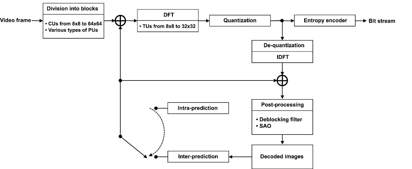
Figure 1. Block diagram of a standard HEVC encoder

It is apparent from the above that the encoding procedure can significantly distort the original image. The distortion is introduced when the spectral coefficients are quantized. The HEVC standard provides an option to apply additional post-processing to the decoded images in order to reduce the effects of quantization. This post-processing can include a deblocking filter (DBF) and a Sample Adaptive Offset (SAO) procedure. Let us explore how this works.

Video image post-processing algorithms in HEVC. Deblocking filter.

The first post-processing stage, the deblocking filter, is designed to reduce edge effects (also known as blockiness, or block effects). During coding, each video frame is divided into equally sized square blocks called Largest Coding Units (LCUs). Each LCU can be divided into four square Coding Units (CUs), each of which can in turn be divided into four more CUs. These divisions result in a CTU (Coding Tree Unit) quadtree. The lowest-level CUs in the CTU are then divided during the coding process into blocks called Prediction Units (PUs).

After that, a 2D spectral transform is applied to the 2D difference signal obtained by subtracting the prediction results from the image being coded. The size of the spectral transform matrix is determined by the size of a Transform Unit (TU). HEVC specifies 4 possible transform unit sizes: 4×4, 8×8, 16×16, and 32×32. The quantization of the spectral coefficients causes blockiness in the decoded images, which is clearly visible in Fig. 2. This figure shows a portion of a decoded image before applying the deblocking filter. For obvious reasons, the effect manifests itself both at the PU and TU boundaries.

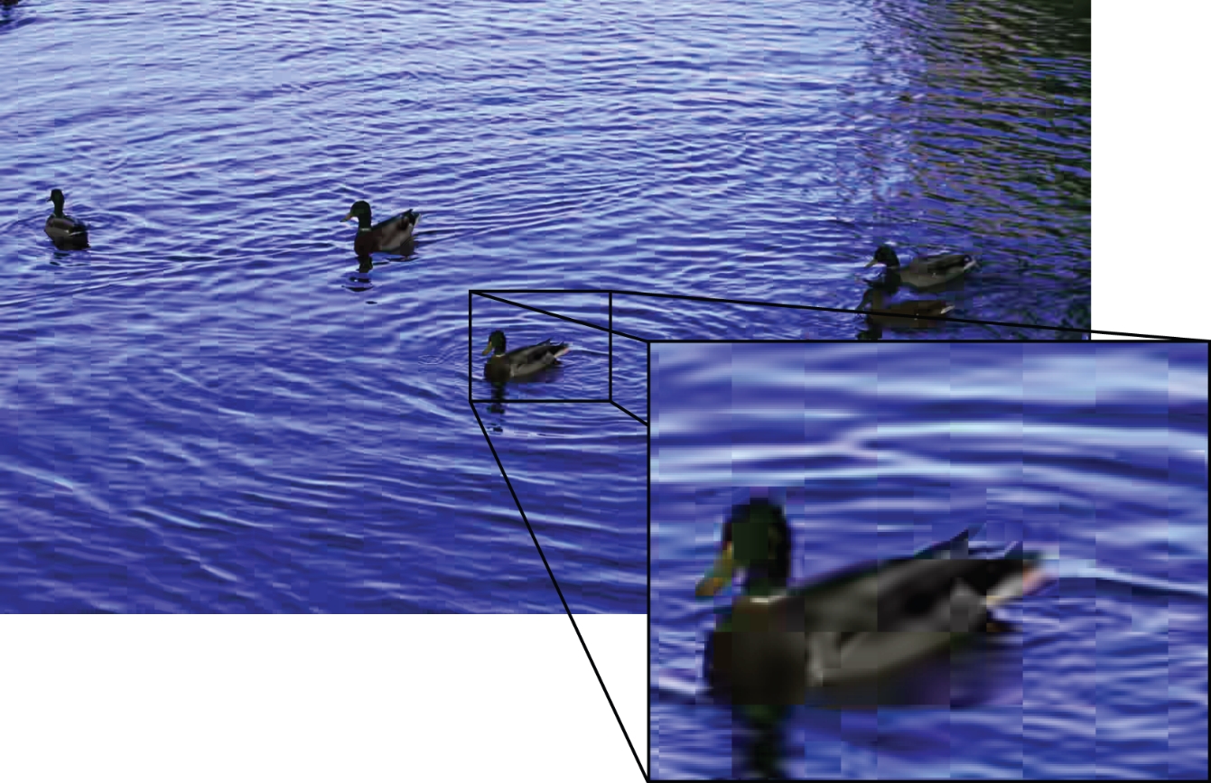
Figure 2. Blockiness effect due to the quantization of spectral coefficients is apparent in the zoomed portion of the video image

The deblocking filtering procedure modifies the values of the pixels located near the vertical and horizontal TU or PU boundary lines, which form an equidistant grid with a pitch of 8 pixels. The filtering is first applied to the vertical lines and then to the horizontal ones.

Before filtering, a value of the Boundary Strength (BS) parameter is chosen for each 4-pixel line segment. This value is determined by the prediction modes used for the image areas on opposite sides of the line segment. If at least one of them was coded using intra-prediction, BS is assigned a value of 2. If both areas were inter-predicted based on one contiguous area of a previously encoded image, the BS parameter for that line segment is assigned a value of 0. Otherwise BS is equal to 1. The areas around the 4-pixel segments where BS = 0 are excluded from the filtering.

The next step involves selecting the filter type as well as the width and position of the area to be filtered. The criterion here is the degree to which the 3×4 -pixel surfaces to the left and right of the boundary deviate from a plane. Let us consider an example of the selection procedure by analyzing an image area in the vicinity of a vertical line segment using the traditional notation (Fig. 3).

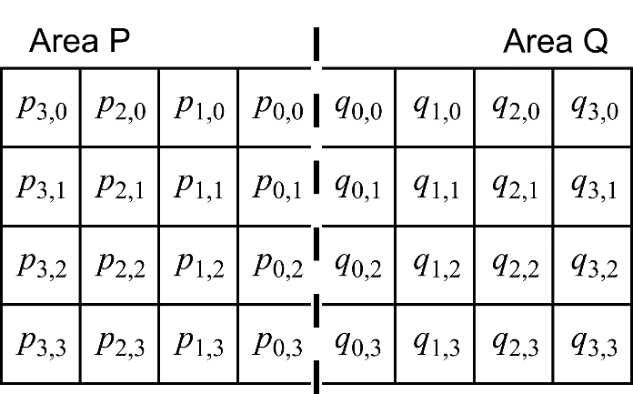
Figure 3. Notation used in the example (the dashed line shows the vertical block boundary)

The area P, located to the left of the boundary, is considered “sufficiently flat”, if the intensity values of the samples in the zero-th and third lines exhibit a near-linear dependency on the horizontal coordinate (distance from the boundary):

$$\begin{array}{l}{p}_{x,0}\approx a_0\cdot x+b_0,p_{x,3}\approx a_3\cdot x+b_3,\end{array}$$

where ${\displaystyle x=0,1,2}$ is the horizontal coordinate. The closeness to a linear relation is estimated by the difference in slope at points ${\displaystyle x=1}$ and ${\displaystyle x=0}$ — that is, by the quantity ${\displaystyle d{p}_0=|\frac{p_{2,0}-p_{1,0}}{2-1}-\frac{p_{1,0}-p_{0,0}}{1-0}|=|p_{2,0}-2p_{1,0}+p_{0,0}|}$ for the upper row pf samples and by ${\displaystyle d{p}_3=|p_{2,3}-2p_{1,3}+p_{0,3}|}$ for the lower row. Corresponding quantities, ${\displaystyle d{q}_0}$ and ${\displaystyle d{q}_3}$, are calculated for the area Q located to the right of the boundary:

$$\begin{array}{l}d{q}_0=|q_{2,0}-2q_{0,1}+q_{0,0}|,d{q}_3=|q_{2,3}-2q_{1,3}+q_{0,3}|\end{array}$$

The decision on the filter type to use as well as the width and position of the area to be smoothed in the vicinity of a boundary is made by comparing various combinations of the quantities ${\displaystyle d{p}_0}$, ${\displaystyle d{p}_3}$, ${\displaystyle d{q}_0}$ and ${\displaystyle d{q}_3}$ with the corresponding threshold values. The threshold values are obtained from the values of ${\displaystyle \beta (Qp)}$ and ${\displaystyle t_C(Qp=2(Bs-1))}$ specified by the standard in the tabular form for each value of quantization parameter ${\displaystyle Qp}$ which determines the quantization step size for the spectral coefficients. The indexing in the table of ${\displaystyle t_C}$ threshold values incorporates the BS parameter.

When sample intensity variation in the vicinity of a boundary is high, i.e. when the following condition is not met:

$$\begin{array}{l}d{p}_0+d{q}_0+d{p}_3+d{q}_3<\beta \end{array}$$

the width of the area to be smoothed is set to zero, and the pixels near the boundary are not filtered (Fig. 4).

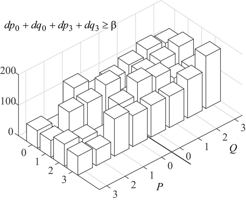
Figure 4. In the case of high sample intensity variation in the vicinity of the boundary, the width of the area to be smoothed is set to zero, and the pixels near the boundary are not filtered

Otherwise, i.e. when

$$\begin{array}{l}d{p}_0+d{q}_0+d{p}_3+d{q}_3<\beta \end{array}$$

a choice is made between “strong” and “weak” filtering. When the following conditions are satisfied:

$$\begin{array}{l}d{p}_0+d{q}_0<\beta /8,\end{array}$$ $$\begin{array}{l}d{p}_3+d{q}_3<\beta /8,\end{array}$$ $$\begin{array}{l}|p_{3,0}-p_{0,0}|+|q_{3,0}-q_{0,0}|<\beta /8,\end{array}$$ $$\begin{array}{l}|p_{3,3}-p_{0,3}|+|q_{3,3}-q_{0,3}|<\beta /8,\end{array}$$ $$\begin{array}{l}|p_{0,0}-q_{0,0}|<2.5t_{C\prime }\end{array}$$ $$\begin{array}{l}|p_{0,3}-q3|<2.5t_C\end{array}$$

the “strong” filter is applied to the vicinity of the boundary. In this case, the area to be smoothed spans 3 samples on each side of the boundary (Fig. 5).

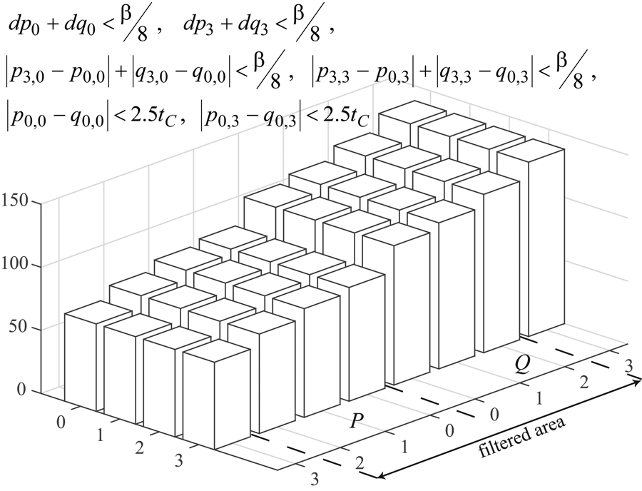
Figure 5. Position of the area to be filtered by “strong” filtering

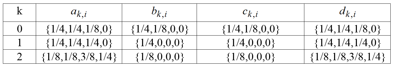
The “strong” filter is applied by row. New values of ${\displaystyle p_{i,j}^n}$ and ${\displaystyle q_{i,j}^n}$ are calculated as linear combinations of samples ${\displaystyle p_{i,j}}$ and ${\displaystyle q_{i,j}}$ in the j-th row:

$$\begin{array}{l}{p}_{k,j}^n=\sum _{i=0}^3{a}_{k,i}{p}_{i,j}+\sum _{i=0}^3{b}_{k,i}{q}_{i,j},\end{array}$$ $$\begin{array}{l}{q}_{k,j}^n=\sum _{i=0}^3{c}_{k,i}{p}_{i,j}+\sum _{i=0}^3{d}_{k,i}{q}_{i,j},j=0,1,2,3;k=0,1,2.\end{array}$$

The values of the coefficients ${\displaystyle a_{k,i}}$, ${\displaystyle b_{k,i}}$, ${\displaystyle c_{k,i}}$, ${\displaystyle d_{k,i}}$ and ${\displaystyle i=0,1,2,3}$ are given in the following table.

When one or more of the conditions in Fig. 5 are not satisfied, i.e. when the “strong” filter is not applicable, the width of the area to be filtered is calculated, and the applicability of the “weak” filter is verified row by row. The number of samples to be smoothed using the “weak” filter is determined independently for the areas P and Q.

If ${\displaystyle d{p}_0+d{p}_3<3/16\beta }$, then for each row in P, the two samples closest to the boundary change their values. Otherwise, just one ${\displaystyle p_{0,j}}$ sample is changed in each row during filtering.

Corresponding conditions must be verified in the Q area. If ${\displaystyle d{q}_0+d{q}_3<3/16\beta }$, then for each row in Q, the two samples closest to the boundary change their values. If this condition is not met, then just one ${\displaystyle q_{0,j}}$ sample is changed in each row during filtering.

New values of samples ${\displaystyle p_{0,j}^n}$, ${\displaystyle p_{1,j}^n}$, ${\displaystyle q_{0,j}^n}$, and ${\displaystyle q_{1,j}^n}$ are calculated based on the quantity ${\displaystyle {△}_j}$:

$$\begin{array}{l}{△}_j=9(q_{0,j}-p_{0,j})-3(q_{1,j}-p_{1,j})\end{array}$$

If ${\displaystyle {△}_j>10t_C(Qp+2(Bs-1))}$, the j-th row is excluded from the filtering, otherwise new values are calculated using the following equations:

$$\begin{array}{l}{p}_{0,j}^n=p_{0,j}+{△}_j\end{array}$$ $$\begin{array}{l}{q}_{0,j}^n=q_{0,j}-{△}_j\end{array}$$ $$\begin{array}{l}{p}_{1,j}^n=p_{1,j}+\frac{\frac{p_{2,j}=p_{0,j}}{2}-p_{1,j}+{△}_j}{2}\end{array}$$ $$\begin{array}{l}{q}_{1,j}^n=q_{1,j}+\frac{\frac{q_{2,j}=q_{0,j}}{2}-q_{1,j}+{△}_j}{2}\end{array}$$

For those who want an in-depth analysis.

The above description of the procedure of applying the deblocking filter does not really explain the nature of the ${\displaystyle a_{k,i}}$, ${\displaystyle b_{k,i}}$, ${\displaystyle c_{k,i}}$ and ${\displaystyle d_{k,i}}$ coefficients used for “strong” filtering and the quantity ${\displaystyle {△}_j}$ used to calculate sample values in the case of “weak” filtering. I was unable to find any derivation of these in the literature. Why are they the way they are? We could speculate a little bit here.

Let us start with ${\displaystyle {△}_j}$. Place the origin of a Cartesian coordinate system in the middle between the samples ${\displaystyle p_{0,j}}$ and ${\displaystyle q_{0,j}}$ so that the coordinates of these samples become ${\displaystyle x=-1/2}$ and ${\displaystyle x=1/2}$, respectively. In this case, the sample ${\displaystyle p_{1,j}}$ has a coordinate of ${\displaystyle x=-3/2}$ and the sample ${\displaystyle q_{1,j}}$ a coordinate of ${\displaystyle x=3/2}$ (Fig. 6).

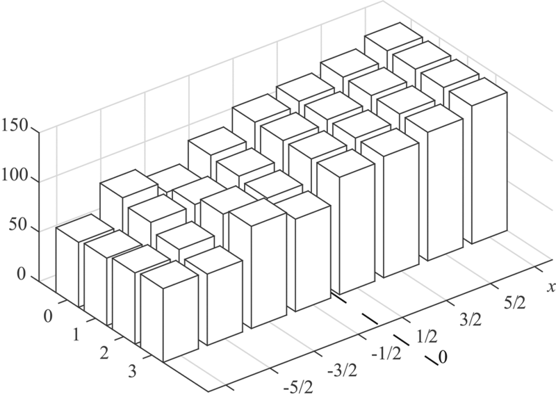
Figure 6. Position and coordinates of samples in a Cartesian coordinate system used for further discussion

Using the least squares method, we draw a straight line ${\displaystyle y=ax+b}$ through the four samples (${\displaystyle p_{0,j}}$, ${\displaystyle p_{1,j}}$, ${\displaystyle q_{0,j}}$, and ${\displaystyle q_{1,j}}$).

The least squares method. Consider a set of samples ${\displaystyle y_i}$ with values taken at points with coordinates ${\displaystyle x_i}$. To approximate ${\displaystyle y_i(x_i)}$ with a linear function, i.e. to construct a straight line with the equation ${\displaystyle y=ax+b}$, we need to choose the values of parameters ${\displaystyle a}$ and ${\displaystyle b}$ so as to minimize the mean square deviation of the ${\displaystyle y_i(x_i)}$ samples from the values given by ${\displaystyle y=a{x}_i+b}$. The extrema of parameters ${\displaystyle a}$ and ${\displaystyle b}$ can be easily found by equating their derivatives to 0:

$$\begin{array}{l}\frac{\partial }{\partial a}\sum _i(y_i-a{x}_i-b{)}^2=0\end{array}$$ $$\begin{array}{l}\frac{\partial }{\partial b}\sum _i(y_i-a{x}_i-b{)}^2=0\end{array}$$

Solving this system of equations for ${\displaystyle a}$ and ${\displaystyle b}$, we obtain:

$$\begin{array}{l}a=\frac{\sum _i{y}_i{x}_i-\sum _i{y}_i\sum _i{x}_i}{\sum _i{x}_i^2-\sum _i{x}_i\sum _i{x}_i}\end{array}$$ , $$\begin{array}{l}b=\sum _i{y}_i-a\sum _i{x}_i\end{array}$$ .

Estimates of ${\displaystyle a}$ and ${\displaystyle b}$ are readily expressed as:

${\displaystyle a=\frac{\sum _i{y}_i{x}_i}{\sum _i{x}_i^2},b=\sum _i{y}_i}$, ${\displaystyle \sum _i{x}_i=0}$. (In the chosen coordinate system, the relation ${\displaystyle \sum _i{x}_i=0}$ holds.)

Substituting the ${\displaystyle x_i}$ coordinates and the ${\displaystyle y_i}$ values into the equations for ${\displaystyle a}$ and ${\displaystyle b}$, we have

<$$\begin{array}{l}a=\frac{-3p_{1,j}-p_{0,j}+q_{0,j}+3q_{1,j}}{10},b=\frac{p_{1,j}+p_{0,j}+q_{0,j}+q_{1,j}}{4}\end{array}$$ .

The deviation of ${\displaystyle p_{0,j}}$ from ${\displaystyle ax+b}$ with ${\displaystyle x=-1/2}$equals

$$\begin{array}{l}△p_{0,j}=p_{0,j}-a(-\frac{1}{2})-b=\frac{-4p_{1,j}+7p_{0,j}-2q_{0,j}-q_{1,j}}{10}\end{array}$$ .

The deviation of ${\displaystyle q_{0,j}}$ from ${\displaystyle ax+b}$ for ${\displaystyle x=1/2}$ equals

$$\begin{array}{l}△q_{0,j}=q_{0,j}-\frac{a}{2}-b=\frac{-p_{1,j}-2p_{0,j}+7q_{0,j}-4q_{1,j}}{10}\end{array}$$ .

The arithmetic mean (taking into account the opposite signs of the deviations ${\displaystyle △p_{0,j}}$ and ${\displaystyle △q_{0,j}}$) given as

$$\begin{array}{l}\frac{△q_{0,j}-△p_{0,j}}{2}=\frac{3p_{1,j}-9p_{0,j}+9q_{0,j}-3q_{2,j}}{20}\end{array}$$

is equal to the ${\displaystyle {△}_j}$ value used for “weak” filtering with an accuracy of 1.25% or better. Thus, the quantity ${\displaystyle {△}_j}$ is determined by the mean deviation of the points ${\displaystyle p_{0,j}}$ and ${\displaystyle q_{0,j}}$ from a straight line drawn using the least squares method through the four points ${\displaystyle p_{1,j}}$, ${\displaystyle q_{0,j}}$ and ${\displaystyle q_{1,j}}$.

Note that the values ${\displaystyle p_{2,j}}$ and ${\displaystyle q_{2,j}}$ are not used at all in drawing the line. If the image in area ${\displaystyle P}$ is sufficiently smooth (i.e. ${\displaystyle d{p}_0+d{p}_3<3/16\beta }$), displacing the ${\displaystyle p_{0,j}}$ sample by ${\displaystyle {△}_j}$ can cause a visible step to appear between ${\displaystyle p_{0,j}}$ and ${\displaystyle p_{1,j}}$. The resulting step is smoothed by adding ${\displaystyle {△}_{1,j}=\frac{\frac{2_{2,j}+p_{0,j}}{2}-p_{1,j}+{△}_j}{2}}$, an easily interpreted quantity, to ${\displaystyle p_{1,j}}$. Indeed, ${\displaystyle △{\prime }_j=\frac{p_{2,j}+p_{0,j}}{2}-p_{1,j}}$ represents the deviation of the ${\displaystyle p_{1,j}}$ value from a straight line drawn through two points, ${\displaystyle p_{0,j}}$ and ${\displaystyle p_{2,j}}$. Therefore, ${\displaystyle {△}_{1,j}=\frac{{△}_j\prime +{△}_j}{2}}$. Adding this to ${\displaystyle p_{1,j}}$ provides a smooth transition from ${\displaystyle p_{0,j}^n=p_{0,j}+{△}_j}$.

A similar smoothing procedure is carried out in area ${\displaystyle Q}$ if it is sufficiently smooth (i.e. when ${\displaystyle d{q}_0+d{q}_3<3/16\beta }$).

With “strong” filtering, new sample values in area P are obtained using the following equations:

$$\begin{array}{l}{p}_{0,j}^n=\frac{p_{2,j}+2p_{1,j}+2p_{0,j}+q_{1,j}}{8}\end{array}$$ , $$\begin{array}{l}{p}_{1,j}^n=\frac{p_{2,j}+p_{1,j}+p_{0,j}+q_{0,j}}{4}\end{array}$$ , $$\begin{array}{l}{p}_{2,j}^n=\frac{2p_{3,j}+3p_{2,j}+p_{1,j}+p_{0,j}+q_{0,j}}{8}\end{array}$$ .

The equation for ${\displaystyle p_{1,j}^n}$ is the easiest to interpret. Indeed, it is simply the arithmetic mean of four values: ${\displaystyle p_{2,j}}$, ${\displaystyle p_{1,j}}$, ${\displaystyle p_{0,j}}$ and ${\displaystyle q_{0,j}}$. The equation for ${\displaystyle p_{0,j}^n}$ can also be viewed as the arithmetic mean of four quantities, ${\displaystyle \frac{p_{2,j}+p_{1,j}}{2}}$, ${\displaystyle \frac{p_{21j}+p_{0,j}}{2}}$, ${\displaystyle \frac{p_{0,j}+q_{0,j}}{2}}$, and ${\displaystyle \frac{q_{0,j}+q_{1,j}}{2}}$, which in turn can be interpreted as the results of linear sample interpolation. The interpolated samples are offset from the original ones by a half-pixel. The equation for ${\displaystyle p_{2,j}^n}$ is the arithmetic mean of two quantities: ${\displaystyle \frac{p_{3,j}+p_{2,j}}{2}}$ and ${\displaystyle p_{1,j}^n}$. Here, taking a mean smooths the transition from ${\displaystyle p_{1,j}^n}$ to the value ${\displaystyle p_{3,j}}$ that stays unchanged during the filtration.

The second stage of post-processing of the decoded images.

This stage is called Sample Adaptive Offset (SAO) and is designed to partially compensate the losses that have occurred due to the quantization of the spectral coefficients. To that end, offsets are added to the values of certain image pixels after decoding. These offsets are calculated at the encoding stage and transmitted in the encoded stream as tables for each LCU. The pixels to be changed are chosen by their intensity, which is why this transformation is non-linear. There are two possible types of SAO in HEVC: Band Offset (BO) and Edge Offset (EO).

For BO post-processing, all pixel values in a LCU are divided into 32 evenly spaced bands at the coding stage. The average offset between the original and decoded image pixels is calculated for each band in the LCU. The video encoder saves the offset values for four consecutive bands and the number of the first band in this quadruple in the encoded stream. After decoding the image at the SAO stage, offsets are added to the pixels whose values fall in the bands chosen by the encoder.

For EO post-processing, the encoder chooses one of four templates according to which the values of the decoded image pixels should be classified. The possible templates are shown in Fig. 4. The sample to be classified is designated as p and the values of the two adjacent samples as n₀ and n₁. The number of the chosen template is added to the encoded stream for each LCU.

Then the sample values are classified into four categories according to that template. If and , then p belongs to the first category. If ( and ) or ( and ), p belongs to the second category. The third category comprises the samples for which ( and ) or ( and ) and the fourth one consists of the samples for which and . For each category of samples, the average difference (offset) from the original values—that is, from the sample values before coding—is calculated during coding and added to the encoded stream. At the post-processing stage, the calculated offsets are added to the decoded sample values. The values of samples that do not fall into any of the four categories are not modified.

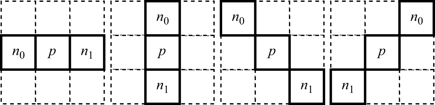
Figure 7. Templates for the classification of sample values

Is post-processing effective?

The results of encoding large numbers of test video sequences make it possible to state that the deblocking filter in the HEVC video coding system is definitely effective. This technique appears particularly useful with high values of the quantization parameter, when the edge effects are especially strong. Decreasing the values of the quantization parameter makes the decoded image less blocky, which in turn reduces the effectiveness of the deblocking filter.

With regard to the effectiveness of the second post-processing stage, however, no such clear conclusion can be drawn. When SAO is used, the encoder inserts additional data into the encoded stream describing the offsets used to correct the decoded image pixel values, which in any case reduces the compression ratio somewhat. On the other hand, enabling SAO improves image quality. As a result, using SAO sometimes provides certain, if modest, gain in terms of compression ratio vs. image quality. However, situations are also possible when the bit rate increase caused by SAO is not compensated by an increase in image quality.

April 1, 2019

Read more:

Chapter 1. Video encoding in simple terms

Chapter 2. Inter-frame prediction (Inter) in HEVC

Chapter 3. Spatial (Intra) prediction in HEVC

Chapter 4. Motion compensation in HEVC

Chapter 6. Context-adaptive binary arithmetic coding. Part 1

Chapter 7. Context-adaptive binary arithmetic coding. Part 2

Chapter 8. Context-adaptive binary arithmetic coding. Part 3

Chapter 9. Context-adaptive binary arithmetic coding. Part 4

Chapter 10. Context-adaptive binary arithmetic coding. Part 5

About the author:

Oleg Ponomarev, 16 years in video encoding and signal digital processing, expert in Statistical Radiophysics, Radio waves propagation.  Assistant Professor, PhD at Tomsk State University, Radiophysics department. Head of Elecard Research Lab.

Use Elecard StreamEye to analyze bitstream

Check the tool to compare encoders